45 labels and values in excel
Excel Chart not showing SOME X-axis labels - Super User Apr 05, 2017 · I have a chart that refreshes after a dataload, and it seems like when there are more than 25 labels on the x-axis, the 26th and on do not show, though all preceding values do. Also, the datapoints for those values show in the chart. In the chart data window, the labels are blank. Any ideas? Custom Chart Data Labels In Excel With Formulas Follow the steps below to create the custom data labels. Select the chart label you want to change. In the formula-bar hit = (equals), select the cell reference containing your chart label's data. In this case, the first label is in cell E2. Finally, repeat for all your chart laebls.
Prevent Overlapping Data Labels in Excel Charts - Peltier Tech May 24, 2021 · Overlapping Data Labels. Data labels are terribly tedious to apply to slope charts, since these labels have to be positioned to the left of the first point and to the right of the last point of each series. This means the labels have to be tediously selected one by one, even to apply “standard” alignments.
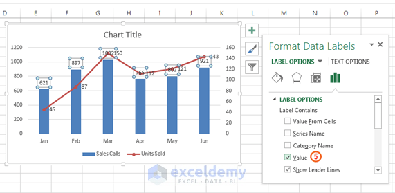
Labels and values in excel
How to Flatten, Repeat, and Fill Labels Down in Excel Summary. Select the range that you want to flatten - typically, a column of labels. Highlight the empty cells only - hit F5 (GoTo) and select Special > Blanks. Type equals (=) and then the Up Arrow to enter a formula with a direct cell reference to the first data label. Instead of hitting enter, hold down Control and hit Enter. Create Dynamic Chart Data Labels with Slicers - Excel Campus Feb 10, 2016 · The next step is to change the data labels so they display the values in the cells that contain our CHOOSE formulas. As I mentioned before, we can use the “Value from Cells” feature in Excel 2013 or 2016 to make this easier. You basically need to select a label series, then press the Value from Cells button in the Format Data Labels menu. What's the difference between 'show labels' and 'show values' in the ... By adding the Scale label type "…,3,2,1" to a question the first answer option will actually get the highest value instead of the lowest. And when you download the raw data with the Show values option you will only see these values, and no text anymore. The 'not applicable' answer option has a fixed value of '99'.
Labels and values in excel. Import variables with label and values - Forums - IBM Support my question is simple: I have an excel file which contains large amount of data, variables, lables and values. a sample file is attached to this message. I create this kind of excel file, by software I developed in Delphi XE. I need to import this file into SPSS. Question 1: is my excel format is correct to import? if not, please advice. How to Find, Highlight, and Label a Data Point in Excel Scatter Plot? By default, the data labels are the y-coordinates. Step 3: Right-click on any of the data labels. A drop-down appears. Click on the Format Data Labels… option. Step 4: Format Data Labels dialogue box appears. Under the Label Options, check the box Value from Cells . Step 5: Data Label Range dialogue-box appears. Excel- Labels, Values, and Formulas - WebJunction Notice also that the labels (composed of letters) are all left justified and the values (composed of numbers) are all right justified in their cells. Simple Formula: Click the cell in which you want the answer (result of the formula) to appear. Press Enter once you have typed the formula. All formulas start with an = sign. Format Data Labels in Excel- Instructions - TeachUcomp, Inc. To format data labels in Excel, choose the set of data labels to format. To do this, click the "Format" tab within the "Chart Tools" contextual tab in the Ribbon. Then select the data labels to format from the "Chart Elements" drop-down in the "Current Selection" button group. Then click the "Format Selection" button that ...
How to Use Cell Values for Excel Chart Labels Mar 12, 2020 · The values from these cells are now used for the chart data labels. If these cell values change, then the chart labels will automatically update. Link a Chart Title to a Cell Value. In addition to the data labels, we want to link the chart title to a cell value to get something more creative and dynamic. How do you show percentage difference in Excel graph? In the opening Format Data Labels pane, check the Percentage box and uncheck the Value box in the Label Options section. Then the percentages are shown in the pie chart as below screenshot shown. ... Create a chart with both percentage and value in Excel. To solve this task in Excel, please do with the following step by step: 1. Select the data ... Understanding Excel Chart Data Series, Data Points, and Data Labels These are commonly used for pie charts. Percentage Labels: Calculated by dividing the individual fields in a series by the total value of the series. Percentage labels are commonly used for pie charts. Data Series: A group of related data points or markers that are plotted in charts and graphs. Examples of a data series include individual lines ... Custom Data Labels with Colors and Symbols in Excel Charts - [How To] To apply custom format on data labels inside charts via custom number formatting, the data labels must be based on values. You have several options like series name, value from cells, category name. But it has to be values otherwise colors won't appear. Symbols issue is quite beyond me.
How to Change Excel Chart Data Labels to Custom Values? 05.05.2010 · This is the only page in a new spreadsheet, created from new, in Win Pro 2010, excel 2010. Cols C & D are values (hard coded, Number format). Col B is all null except for “1” in each cell next to the labels, as a helper series, iaw a web forum fix. Col A is x axis labels (hard coded, no spaces in strings, text format), with null cells in ... How to create label cards in Excel - Ablebits Select By empty row to separate groups of records with blank rows. If you choose to get more than one column with the results, you can also divide them By empty column. Save original headers and formatting: Tick the Add header checkbox to display all column headers as labels next to the values in your cards. How to Print Labels From Excel - Lifewire Select Mailings > Write & Insert Fields > Update Labels . Once you have the Excel spreadsheet and the Word document set up, you can merge the information and print your labels. Click Finish & Merge in the Finish group on the Mailings tab. Click Edit Individual Documents to preview how your printed labels will appear. Select All > OK . Add a label or text box to a worksheet Add a label (Form control) Click Developer, click Insert, and then click Label . Click the worksheet location where you want the upper-left corner of the label to appear. To specify the control properties, right-click the control, and then click Format Control. Add a label (ActiveX control) Add a text box (ActiveX control) Show the Developer tab
Excel Chart Elements: Parts of Charts in Excel | ExcelDemy
What is the difference between spreadsheet labels and values ... - Answers What is the difference of a number and a label in excel? Labels are normally headings over cells that have values in them. So in A1 you could have the word Sales. From A2 down you would have...
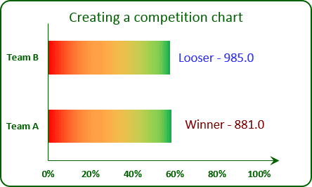
Creating a chart with dynamic labels - Microsoft Excel 2013
Excel tutorial: How to use data labels You can set data labels to show the category name, the series name, and even values from cells. In this case for example, I can display comments from column E using the "value from cells" option. Leader lines simply connect a data label back to a chart element when it's moved. You can turn them off if you want.

Excel: Grouping pivot table entries
How to add data labels from different column in an Excel chart? In the Format Data Labels pane, under Label Options tab, check the Value From Cells option, select the specified column in the popping out dialog, and click the OK button. Now the cell values are added before original data labels in bulk. 4. Go ahead to untick the Y Value option (under the Label Options tab) in the Format Data Labels pane.
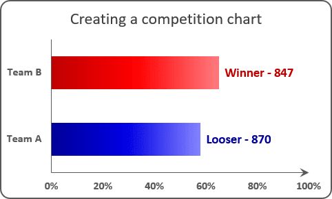
Creating a chart with dynamic labels - Microsoft Excel 2016
The Art of Dynamic Labeling in Excel - dummies On the Insert tab in the Ribbon, select the Text Box icon. Click inside the chart to create an empty text box. While the text box is selected, go up to the formula bar, type the equal sign (=), and then click the cell that contains the text for your dynamic label. The text box is linked to cell C2. You'll notice that cell C2 holds the Filter ...
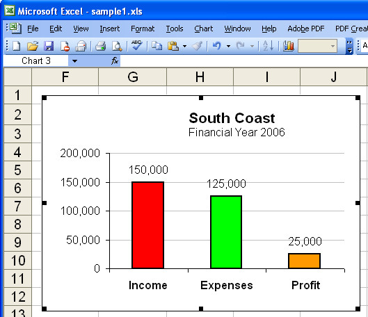
31 What Is A Label In Excel - Labels For Your Ideas
Text Labels on a Horizontal Bar Chart in Excel - Peltier Tech Dec 21, 2010 · In this tutorial I’ll show how to use a combination bar-column chart, in which the bars show the survey results and the columns provide the text labels for the horizontal axis. The steps are essentially the same in Excel 2007 and in Excel 2003. I’ll show the charts from Excel 2007, and the different dialogs for both where applicable.
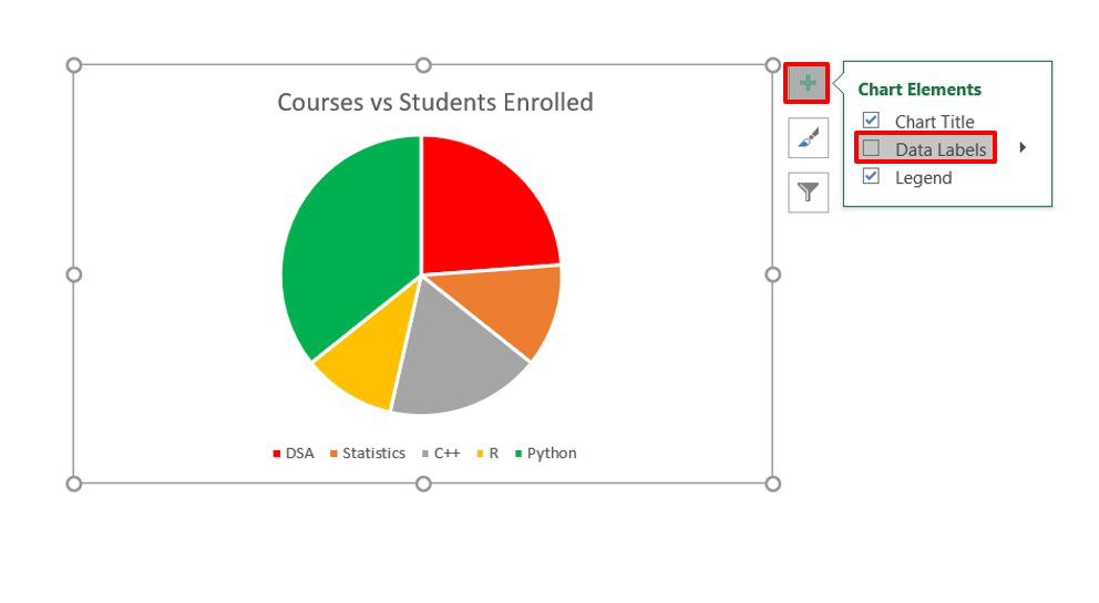
How to Show Percentage in Pie Chart in Excel? - GeeksforGeeks
DOC Excel - WebJunction Excel. Labels, Values & Formulas . Labels and values . Entering data into a spreadsheet is just like typing in a word processing program, but you have to first click the cell in which you want the data to be placed before typing the data. All words describing the values (numbers) are called labels. The numbers, which can later be used in ...

Excel Tutorials - My Two Bits of Information
How to group (two-level) axis labels in a chart in Excel? (1) In Excel 2007 and 2010, clicking the PivotTable > PivotChart in the Tables group on the Insert Tab; (2) In Excel 2013, clicking the Pivot Chart > Pivot Chart in the Charts group on the Insert tab. 2. In the opening dialog box, check the Existing worksheet option, and then select a cell in current worksheet, and click the OK button. 3.
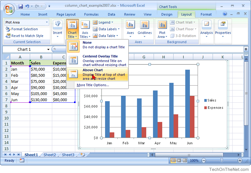
MS Excel 2007: How to Create a Column Chart
How to Change Excel Chart Data Labels to Custom Values? Define the new data label values in a bunch of cells, like this: Now, click on any data label. This will select "all" data labels. Now click once again. At this point excel will select only one data label. Go to Formula bar, press = and point to the cell where the data label for that chart data point is defined.

Excel 2013: Labels, Values, & Formulas - YouTube
How to Add Labels to Scatterplot Points in Excel - Statology Step 3: Add Labels to Points Next, click anywhere on the chart until a green plus (+) sign appears in the top right corner. Then click Data Labels, then click More Options… In the Format Data Labels window that appears on the right of the screen, uncheck the box next to Y Value and check the box next to Value From Cells.
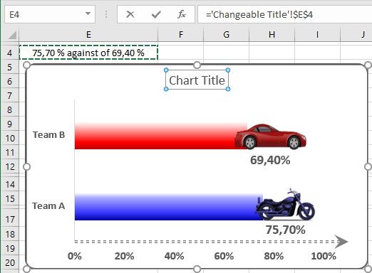
How to create dependent on a volume chart title - Microsoft Excel 2016
Add or remove data labels in a chart - support.microsoft.com Click Label Options and under Label Contains, select the Values From Cells checkbox. When the Data Label Range dialog box appears, go back to the spreadsheet and select the range for which you want the cell values to display as data labels. When you do that, the selected range will appear in the Data Label Range dialog box. Then click OK.

Surface Chart in Excel
Excel Chart Vertical Axis Text Labels • My Online Training Hub Hide the left hand vertical axis: right-click the axis (or double click if you have Excel 2010/13) > Format Axis > Axis Options: Set tick marks and axis labels to None; While you’re there set the Minimum to 0, the Maximum to 5, and the Major unit to 1. This is to suit the minimum/maximum values in your line chart.
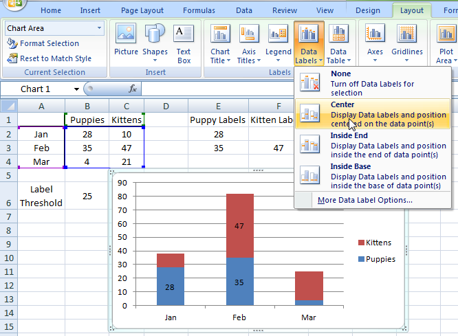
How-to Make Conditional Label Values in an Excel Stacked Column Chart - Excel Dashboard Templates
How to Use Excel Pivot Table Label Filters Right-click a cell in the pivot table, and click PivotTable Options. Click the Totals & Filters tab Under Filters, add a check mark to 'Allow multiple filters per field.' Click OK Quick Way to Hide or Show Pivot Items Easily hide or show pivot table items, with the quick tip in this video. The written instructions are below the video
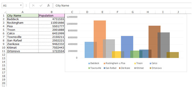
Displaying Numbers in Thousands in a Chart in Microsoft Excel
How to Customize Your Excel Pivot Chart Data Labels - dummies If you want to label data markers with a category name, select the Category Name check box. To label the data markers with the underlying value, select the Value check box. In Excel 2007 and Excel 2010, the Data Labels command appears on the Layout tab. Also, the More Data Labels Options command displays a dialog box rather than a pane.

31 Definition Of Label In Excel - Labels 2021
How to add Axis Labels (X & Y) in Excel & Google Sheets This tutorial will explain how to add Axis Labels on the X & Y Axis in Excel and Google Sheets. How to Add Axis Labels (X&Y) in Excel. Graphs and charts in Excel are a great way to visualize a dataset in a way that is easy to understand. The user should be able to understand every aspect about what the visualization is trying to show right away ...
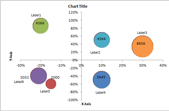
Bubble Charts - Negative Values in X-Axis and Multiple Bubble Colors in UI for ASP.NET AJAX ...
How to Use Cell Values for Excel Chart Labels Select the chart, select the "Chart Elements" alternative, click the "Data Labels" arrow, and then "More Options." Uncheck the "Value" box and examine the "Value From Cells" box. Select cells C2: C6 to use for the information label range and after that click the "OK" button. The values from these cells are now used for the chart data labels.
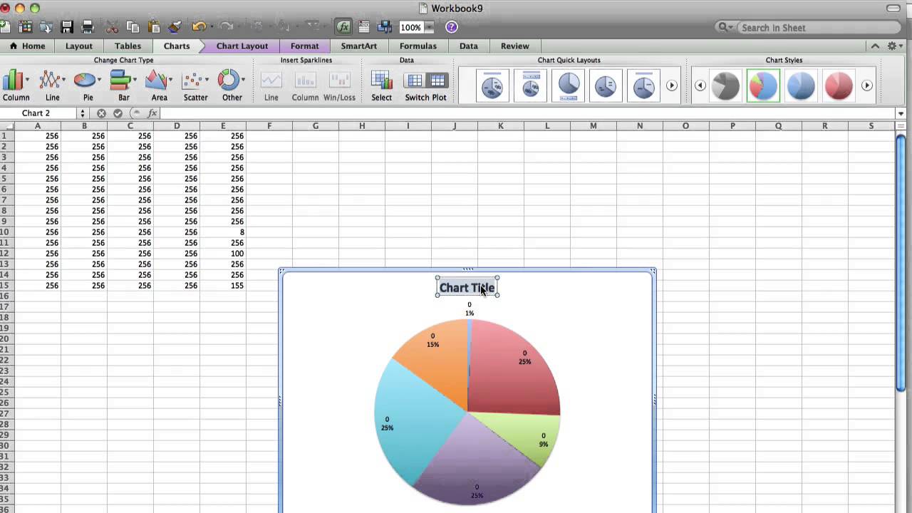
How to Change Excel Chart Name - YouTube
Excel charts: add title, customize chart axis, legend and data labels ... Click the Chart Elements button, and select the Data Labels option. For example, this is how we can add labels to one of the data series in our Excel chart: For specific chart types, such as pie chart, you can also choose the labels location. For this, click the arrow next to Data Labels, and choose the option you want.
Post a Comment for "45 labels and values in excel"