41 how to customize data labels in excel

Custom Excel number format - Ablebits.com To create a custom Excel format, open the workbook in which you want to apply and store your format, and follow these steps: Select a cell for which you want to create custom formatting, and press Ctrl+1 to open the Format Cells dialog. Under Category, select Custom. Type the format code in the Type box. How do I create a one variable data table in Excel? In Excel 2016 for Mac: Click Data > What-if Analysis > Data Table. In Excel for Mac 2011: On the Data tab, under Analysis, click What-If, and then click Data Table. In the Row input cell box, enter the reference to the input cell for the input values in the row.

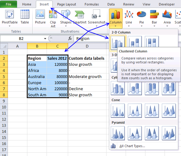
chandoo.org › wp › change-data-labels-in-chartsHow to Change Excel Chart Data Labels to Custom Values? May 05, 2010 · Change Data Labels in Charts to Whatever you want [Quick Tip] First add data labels to the chart (Layout Ribbon > Data Labels) Define the new data label values in a bunch of cells, like this: Now, click on any data label. This will select “all” data labels. Now click once again. At this point excel ...

How to customize data labels in excel

How to Create a Run Chart in Excel (2021 Guide) | 2 Free Templates Go to the Insert tab. Click " Insert Line or Area Chart .". Choose " Line .". You now have your simple run chart as a result: Step 3. Spruce Up Your Run Chart. Technically, you're good to go, but if you're looking to improve your chart from boring to beautiful in mere moments, here's how you can quickly spruce it up. support.microsoft.com › en-us › officeEdit titles or data labels in a chart - support.microsoft.com The first click selects the data labels for the whole data series, and the second click selects the individual data label. Right-click the data label, and then click Format Data Label or Format Data Labels. Click Label Options if it's not selected, and then select the Reset Label Text check box. Top of Page How to Create and Customize a Waterfall Chart in Microsoft Excel Then, use the Fill & Line, Effects, and Size & Properties tabs to do things like add a border, apply a shadow, or scale the chart. Select the chart and use the buttons on the right (Excel on Windows) to adjust Chart Elements like labels and the legend, or Chart Styles to pick a theme or color scheme. Select the chart and go to the Chart Design tab.

How to customize data labels in excel. Pivot Chart Data Label Formatting Question - Microsoft Tech Community Hi, I have a pivot chart. I format the data labels, for example make the text larger or turn it. Every time I refresh the data the data label formatting reverts to the default. I have gone to the Pivot Chart options and made sure the Preserve cell formatting option is checked. How to I get around... How to Print Labels From Excel - Lifewire Choose Start Mail Merge > Labels . Choose the brand in the Label Vendors box and then choose the product number, which is listed on the label package. You can also select New Label if you want to enter custom label dimensions. Click OK when you are ready to proceed. Connect the Worksheet to the Labels How to Make and Print Labels from Excel with Mail Merge How to mail merge labels from Excel . Open the "Mailings" tab of the Word ribbon and select "Start Mail Merge > Labels…". The mail merge feature will allow you to easily create labels ... How to Make a Fillable Form in Excel (5 Suitable Examples) First, go to your OneDrive account and select New >> Forms for Excel After that, give your form a name. Later, add a section by clicking Add new. You will see some form options after that. Suppose you want to insert names first. So you should select Text. After that, type Name as the number one option. Then you can put other options.

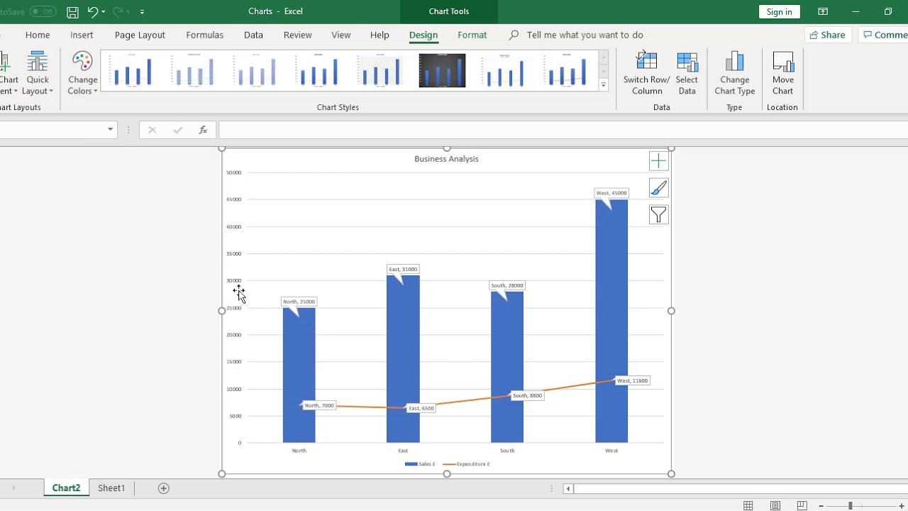
Change the Font Size, Color, and Style of an Excel Form Control Label A look through some Excel forums shows suggestions to use a TextBox shape or an ActiveX Label instead of the hapless Label control.It's a tragedy since the other form controls are lightweight and easy to use. Some forum posters even said Labels are best used to cover cells you don't want the user to click. So sad. How to customize the export to Excel - OutSystems Answer. To customize the name and order of columns/Attributes when exporting a List to an Excel file follow these steps: In the Data tab, create a Structure ( ReceiptsExport) and add the following Attributes: Store: set the Data Type to Text. DateandTime: set the Label to Date and Time and the Data Type to Date Time. How to Add Total Values to Stacked Bar Chart in Excel Step 4: Add Total Values. Next, right click on the yellow line and click Add Data Labels. Next, double click on any of the labels. In the new panel that appears, check the button next to Above for the Label Position: Next, double click on the yellow line in the chart. In the new panel that appears, check the button next to No line: How to mail merge and print labels from Excel - Ablebits In the dialog box that pops up, specify which labels you want to edit. When you click OK, Word will open the merged labels in a separate document. You can make any edits there, and then save the file as a usual Word document. How to make a custom layout of mailing labels

› article › technologyHow to Customize Your Excel Pivot Chart Data Labels - dummies Mar 26, 2016 · If you want to specify what Excel should use for the data label, choose the More Data Labels Options command from the Data Labels menu. Excel displays the Format Data Labels pane. Check the box that corresponds to the bit of pivot table or Excel table information that you want to use as the label. Chart.ApplyDataLabels method (Excel) | Microsoft Docs expression. ApplyDataLabels ( Type, LegendKey, AutoText, HasLeaderLines, ShowSeriesName, ShowCategoryName, ShowValue, ShowPercentage, ShowBubbleSize, Separator) expression A variable that represents a Chart object. Parameters Example This example applies category labels to series one on Chart1. VB Copy Charts ("Chart1").SeriesCollection (1). add custom data labels in Excel Archives - Data Cornering Tag: add custom data labels in Excel. DataViz Excel. How to create a magic quadrant chart in Excel. by Janis Sturis June 22, 2022 Comments 0. Categories. How to format axis labels individually in Excel - SpreadsheetWeb Double-clicking opens the right panel where you can format your axis. Open the Axis Options section if it isn't active. You can find the number formatting selection under Number section. Select Custom item in the Category list. Type your code into the Format Code box and click Add button. Examples of formatting axis labels individually

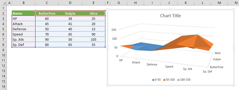
Surface Chart in Excel

How to Create an Automated Data Entry Form in Excel VBA Once you've placed the button, rename it. Right-click on it, and click on New to assign a new macro to show the form.. Enter the following code in the editor window: Sub Button1_Click() UserForm.Show End Sub. Once the Home and Student Database sheets are ready, it's time to design the user form. Navigate to the Developer tab, and click on Visual Basic to open the Editor.

Formula Friday - Using Formulas To Add Custom Data Labels To Your Excel Chart - How To Excel At ...

Custom Chart Data Labels In Excel With Formulas Jan 07, 2022 · Follow the steps below to create the custom data labels. Select the chart label you want to change. In the formula-bar hit = (equals), select the cell reference containing your chart label’s data. In this case, the first label is in cell E2. Finally, repeat for all your chart laebls.

How to Add Data Labels in Excel - Excelchat | Excelchat

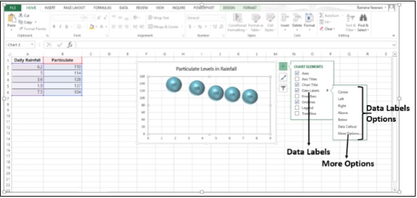
Excel: How to Create a Bubble Chart with Labels - Statology Step 3: Add Labels. To add labels to the bubble chart, click anywhere on the chart and then click the green plus "+" sign in the top right corner. Then click the arrow next to Data Labels and then click More Options in the dropdown menu: In the panel that appears on the right side of the screen, check the box next to Value From Cells within ...

Excel Course: Inserting Graphs

How Do I Create Avery Labels From Excel? - Ink Saver Arrange the fields: Next, arrange the columns and rows in the order they appear in your label. This step is optional but highly recommended if your designs look neat. For this, just double click or drag and drop them in the text box on your right. Don't forget to add commas and spaces to separate fields

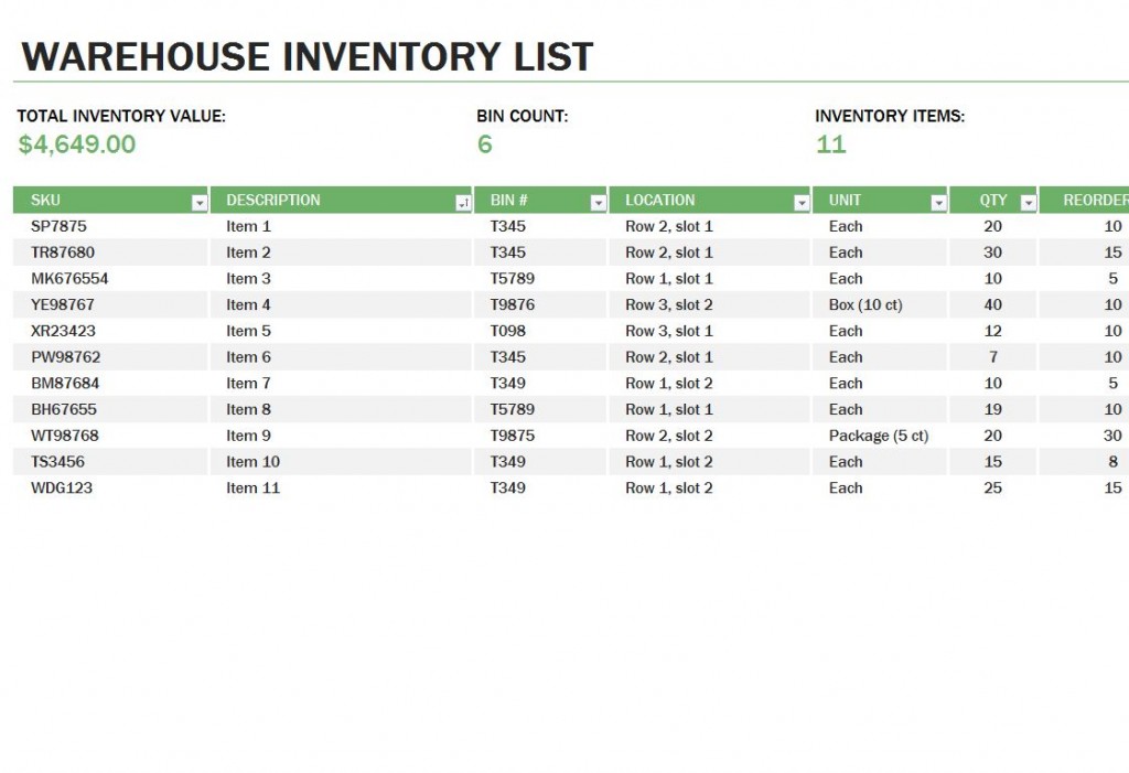
Warehouse Inventory | Warehouse Inventory Template

Manage sensitivity labels in Office apps - Microsoft Purview ... Set Use the Sensitivity feature in Office to apply and view sensitivity labels to 0. If you later need to revert this configuration, change the value to 1. You might also need to change this value to 1 if the Sensitivity button isn't displayed on the ribbon as expected. For example, a previous administrator turned this labeling setting off.

How To Add Data Labels To A Chart in Microsoft Excel - YouTube

Modifying Axis Scale Labels (Microsoft Excel) Follow these steps: Create your chart as you normally would. Double-click the axis you want to scale. You should see the Format Axis dialog box. (If double-clicking doesn't work, right-click the axis and choose Format Axis from the resulting Context menu.) Make sure the Number tab is displayed. (See Figure 1.)

Improve Data Visualization By Mapping with Microsoft Excel | Pressat

How To Add Data Labels In Excel | Nabludatel After moving the data labels to the center in this example, the graph is able to give more information about each of the x axis series. Press f2 to move focus to the formula editing box. Source: . Change position of data labels. Excel provides several options for the placement and formatting of data labels. Source: www ...

How to Create Multi-Category Chart in Excel - Excel Board

How to Create and Customize a Treemap Chart in Microsoft Excel Select the data for the chart and head to the Insert tab. Click the "Hierarchy" drop-down arrow and select "Treemap." The chart will immediately display in your spreadsheet. And you can see how the rectangles are grouped within their categories along with how the sizes are determined.

Excel Video 77 Data Labels - YouTube

How to add text labels on Excel scatter chart axis - Data Cornering Select recently added labels and press Ctrl + 1 to edit them. Add custom data labels from the column "X axis labels". Use "Values from Cells" like in this other post and remove values related to the actual dummy series. Change the label position below data points. Hide dummy data series markers by switching marker options to none.

Custom data labels in a chart | Get Digital Help - Microsoft Excel resource

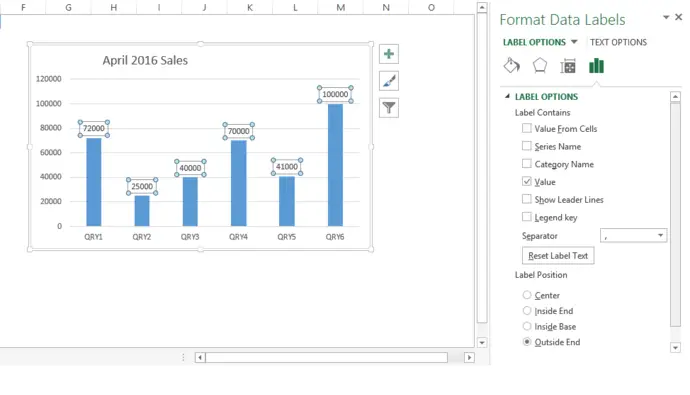
efficiency365.com › 2016/03/01 › describe-the-chartHow to create Custom Data Labels in Excel Charts Mar 01, 2016 · Two ways to do it. Click on the Plus sign next to the chart and choose the Data Labels option. We do NOT want the data to be shown. To customize it, click on the arrow next to Data Labels and choose More Options … Unselect the Value option and select the Value from Cells option. Choose the third column (without the heading) as the range.

Directly Labeling Excel Charts | PolicyViz

Stacked Bar Chart in Power BI [With 27 Real Examples] The stacked bar chart is used to compare Multiple dimensions against a single measure. In the Stacked bar chart, the data value will be represented on the Y-axis and the axis represents the X-axis value. In this example, we use the SharePoint List as the data source to demonstrate the stacked bar chart in Power BI.

How to Print Labels from Excel

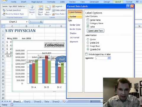
› format-data-labels-in-excelFormat Data Labels in Excel- Instructions - TeachUcomp, Inc. Nov 14, 2019 · To format data labels in Excel, choose the set of data labels to format. To do this, click the “Format” tab within the “Chart Tools” contextual tab in the Ribbon. Then select the data labels to format from the “Chart Elements” drop-down in the “Current Selection” button group.

Advanced Excel - Краткое руководство - CoderLessons.com

support.microsoft.com › en-us › officeChange the format of data labels in a chart To format data labels, select your chart, and then in the Chart Design tab, click Add Chart Element > Data Labels > More Data Label Options. Click Label Options and under Label Contains, pick the options you want. To make data labels easier to read, you can move them inside the data points or even outside of the chart.

Matrix bubble chart with Excel - E90E50fx

How To Create a Header Row in Excel Using 3 Methods 1. Open a spreadsheet and click "View". First, open Excel and choose the spreadsheet that you'd like to edit if you have one with data already entered, or you can choose a new document by clicking the "New" tab and selecting "Blank workbook." Add data to the spreadsheet before you create your header row.

How to Add Data Labels in Excel - Excelchat | Excelchat

Label Excel Vba To Userform Add Dynamically Search: Excel Vba Dynamically Add Label To Userform. Double click on the cancel button from the userform to open the view code for the command button and replace the code with the Unload Me statement as follows Automated Data Entry Form - Part 5 (with Full Screen, Zoom and Dynamic Drop-down) In Part 5, you will learn how to run the Data Entry form in Full Screen and zoom in the controls in ...

It Asset Tracking Spreadsheet — db-excel.com

How to Create and Customize a Waterfall Chart in Microsoft Excel Then, use the Fill & Line, Effects, and Size & Properties tabs to do things like add a border, apply a shadow, or scale the chart. Select the chart and use the buttons on the right (Excel on Windows) to adjust Chart Elements like labels and the legend, or Chart Styles to pick a theme or color scheme. Select the chart and go to the Chart Design tab.

Create a Line Chart in Excel - Easy Excel Tutorial

support.microsoft.com › en-us › officeEdit titles or data labels in a chart - support.microsoft.com The first click selects the data labels for the whole data series, and the second click selects the individual data label. Right-click the data label, and then click Format Data Label or Format Data Labels. Click Label Options if it's not selected, and then select the Reset Label Text check box. Top of Page