42 conditional formatting data labels excel
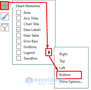
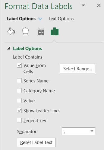
How to use conditional formatting to highlight differences between two ... but still it sometimes highlights the same data (ie both both say '1'), sometimes differences are highlighted (correct), and sometimes it doesn't highlight the difference. ... Labels: Labels: Excel ... Can you attach a screenshot which shows the data and the manager for conditional formatting? A screenshot like the one in my last reply. 0 Likes ... Format Data Labels in Excel- Instructions - TeachUcomp, Inc. To format data labels in Excel, choose the set of data labels to format. To do this, click the "Format" tab within the "Chart Tools" contextual tab in the Ribbon. Then select the data labels to format from the "Chart Elements" drop-down in the "Current Selection" button group. Then click the "Format Selection" button that ...
Conditional formatting with formulas (10 examples) | Exceljet You can create a formula-based conditional formatting rule in four easy steps: 1. Select the cells you want to format. 2. Create a conditional formatting rule, and select the Formula option. 3. Enter a formula that returns TRUE or FALSE. 4. Set formatting options and save the rule. The ISODD function only returns TRUE for odd numbers, triggering the rule:
Conditional formatting data labels excel
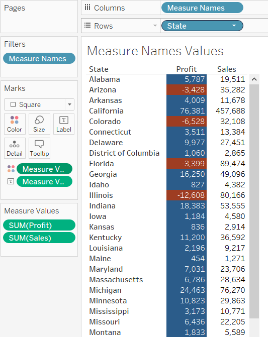
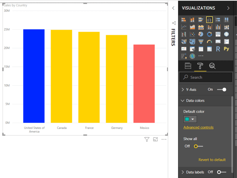
Conditional formatting for Data Labels in Power BI Where you can find the conditional formatting options? Select the visual > Go to the formatting pane> under Data labels > Values > Color Data Labels Let's Get Started- Add one line chart visual into page and create two measure for Profit & Sales. Note: If you don't want to create measure then you can directly use Sales and Profit fields. How To Use Conditional Formatting in Excel in 5 Steps 4. Select an option from the drop-down menu. Once you select the "Conditional Formatting" button, Excel displays several options, starting with "Highlight Cells Rules" and ending with "Manage Rules." Selecting one option from the first five allows you to develop rules based on the option you choose. Using Conditional Formatting to Identify Date-Based Patterns in Excel In the New Formatting Rule box, select "Use a formula to determine which cells to format" as the rule type. Choose "Use a formula to determine which cells to format" to set custom date-based formatting. Enter the formula for the dates you want to highlight in the following format: "=TODAY ()-A1>X" where A1 is the cell number of the first cell ...
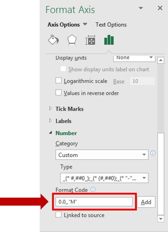
Conditional formatting data labels excel. Changing the Color of a Data Label using IF Statement Highlight a Specific Data Label in an Excel Chart - Peltier Tech Blog Now, it is important to note that Conditional Formatting did not work as it is greyed out for data labels. I even tried Conditional Formatting in the source data and that didn't work either. A few hours later, I came across something interesting. How to do conditional formatting of a label in Excel VBA The TEXT worksheet function seems to respect the format you initially specified and you can use it in your VBA by virtue of Application.WorksheetFunction.. Application.WorksheetFunction.Text(812, "[>=1000000] $#,##0.0,,""M"";[>0] $#,##0.0, ""K"";General") The VBA reference for FORMAT doesn't cover conditional number formatting but it does have a number formatting section, so I expect ... How to Create Excel Charts (Column or Bar) with Conditional Formatting ... The formula puts together a neatly-looking dynamic label based on the previously set conditional formatting rules. The TEXT function formats the values as currency. But if your data type differs, apply this formula instead: =C1&": from "&TEXT(C2, "#,##")&" to "&TEXT(C3, "#,##") Or this one when you work with percentages: Conditionally formatted data: Examples and guidelines Conditionally formatted data: Examples and guidelines Excel 2010 Excel 2007 Enhancements to conditional formatting are a popular feature in Microsoft Excel. Analyzing data has never been more interesting and colorful. Now, you can track trends, check status, spot data, and find top values like never before.
How to Apply Different Types of Conditional Formatting in Excel How to Apply Data Bars Conditional Formatting in Excel. The third type of conditional formatting in Excel is Data Bars. So this will create bars in our data set representing both the positive and negative values. And to apply this type of conditional formatting in Excel, let's learn the following steps below: 1. Firstly, select the needed ... Excel Data Analysis - Conditional Formatting - tutorialspoint.com Follow the steps to conditionally format cells − Select the range to be conditionally formatted. Click Conditional Formatting in the Styles group under Home tab. Click Highlight Cells Rules from the drop-down menu. Click Greater Than and specify >750. Choose green color. Click Less Than and specify < 500. Choose red color. Use conditional formatting to highlight information On the Home tab, in the Styles group, click the arrow next to Conditional Formatting, and then click Manage Rules. The Conditional Formatting Rules Manager dialog box appears. The conditional formatting rules for the current selection are displayed, including the rule type, the format, the range of cells the rule applies to, and the Stop If True setting. A Quick Guide to Conditional Formatting in Excel - HubSpot The image below is the sample data set I'll use for this explanation: 1. First, select column B. 2. Navigate to the header toolbar and select Conditional Formatting. When the Conditional Formatting drop-down menu appears, select Highlight Cells Rules, then Equal To. 3. In the New Formatting dialog box, select Cell Value and Equal To.
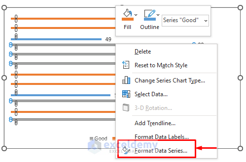
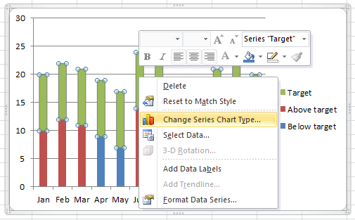
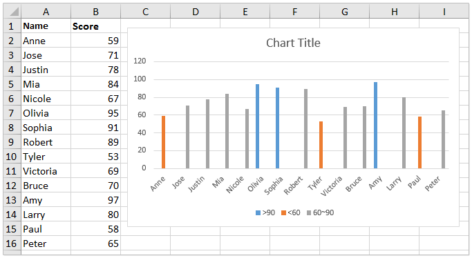
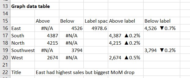
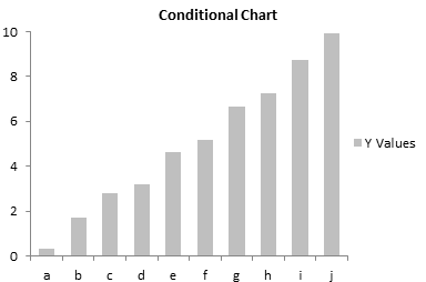
Excel bar chart with conditional formatting based on MoM change Click on any bar and press Ctrl+1 to make the Format Data Series task pane appear if it is not already showing. In the Series Options section, set the Gap Width to 50% to give the bars more presence and set the Series Overlap to 100%. Use the chart skittle (the "+" sign to the right of the chart) to remove the legend and gridlines. r/excel - Is it possible to conditionally format Data Labels on a ... On a dynamic line chart, where Y-axis is scaled from 0-10 and X-axis is dates, is it possible to conditionally format Data Labels such that the colour of the data labels changes based on the data values that are plotted. For example, when numbers 0-3 are plotted on the dynamic chart above their data label's font colour turns red, and if numbers ... Excel tutorial: How to add a conditional formatting key The first step is to create the basic layout for the key. For this, we'll set up a small table with three rows - one for each conditional format. We can then add labels for each conditional format rule. These could be anything, but let's use Excellent, Concern, and Danger. Now let's add the threshold values to the table. How to create a chart with conditional formatting in Excel? - ExtendOffice Add three columns right to the source data as below screenshot shown: (1) Name the first column as >90, type the formula =IF (B2>90,B2,0) in the first blank cell of this column, and then drag the AutoFill Handle to the whole column;
Dynamic Number Format for Millions and Thousands - PK: An ...
Custom Chart Data Labels In Excel With Formulas - How To Excel At Excel Follow the steps below to create the custom data labels. Select the chart label you want to change. In the formula-bar hit = (equals), select the cell reference containing your chart label's data. In this case, the first label is in cell E2. Finally, repeat for all your chart laebls.
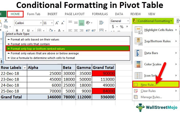
How to Apply Conditional Formatting in Pivot Table? (with ...
Conditional Formatting in Excel - a Beginner's Guide Excel has a tool that automatically helps you out with that — it’s called conditional formatting. If you’re ready to take your data organization game to the next level, keep reading to learn how to use conditional formatting in Excel. In this resource, we'll apply conditional formatting to a pivot table. Note that the steps to apply pivot ...

Change the format of data labels in a chart
How to change chart axis labels' font color and size in Excel? Sometimes, you may want to change labels' font color by positive/negative/ in an axis in chart. You can get it done with conditional formatting easily as follows: 1. Right click the axis you will change labels by positive/negative/0, and select the Format Axis from right-clicking menu. 2. Do one of below processes based on your Microsoft Excel version:

Color Negative Chart Data Labels in Red with downward arrow
Conditional formatting chart data labels? - Excel Help Forum You can use a dummy line chart series to add data labels which can be individually formatted, as I explain in Individually Formatted Category Axis Labels. The easy way to conditionally format these labels is use two series. Use something like =IF($E2=1,0,NA()) for the series that has red labels and =IF(#E2=1,NA(),0) for the series that has unformatted labels.
Excel Bar Graph Color with Conditional Formatting (3 Suitable ...
Conditional Formatting with Data Validation - Microsoft Tech Community On the Home tab of the ribbon, select Conditional Formatting > New Rule... Select 'Use a formula to determine which cells to format'. Enter the formula =AND($A2="value1",$B2="value2",$C2="") Click Format... Activate the Fill tab. Select red. Click OK, then click OK again.

Custom Excel Chart Label Positions • My Online Training Hub
Excel conditional formatting Icon Sets, Data Bars and Color Scales Select all cells in column A, except for the column header, and create a conditional formatting icon set rule by clicking Conditional Formatting > Icon sets > More Rules... In the New Formatting Rule dialog, select the following options: Click the Reverse Icon Order button to change the icons' order. Select the Icon Set Only checkbox.
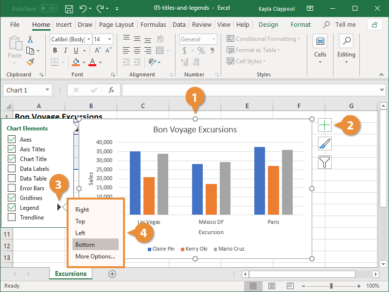
How to Edit a Legend in Excel | CustomGuide
Creating Conditional Data Labels in Excel Charts - YouTube We can make labels appear on our charts that don't have to do with the raw numbers that built the chart - and we can make them show up or not based on whatever conditions we want. In this tutorial,...
Create charts with conditional formatting – User Friendly
Change the format of data labels in a chart To get there, after adding your data labels, select the data label to format, and then click Chart Elements > Data Labels > More Options. To go to the appropriate area, click one of the four icons ( Fill & Line, Effects, Size & Properties ( Layout & Properties in Outlook or Word), or Label Options) shown here.

How to create a chart with conditional formatting in Excel?
Conditional Formatting in Excel - Step by Step Examples - WallStreetMojo The steps to highlight duplicates in the given range are listed as follows: Step 1: From the "conditional formatting" drop-down in the Home tab, select "highlight cells rules.". Choose the option "duplicate values," as shown in the following image. Step 2: The "duplicate values" window appears.

Conditional Formatting of Data Labels on Chart - Microsoft ...
VBA Conditional Formatting of Charts by Value and Label The category labels (XValues) and values (Values) are put into arrays, also for ease of processing. The code then looks at each point's value and label, to determine which cell has the desired formatting. The rows and columns are looped starting at 2, since the first of each contains an irrelevant label. The looping stops one count before the end.
How to create a chart with conditional formatting in Excel?
Apply Conditional Formatting to Data Labels - Power BI Docs Power BI - Excel Sample Data Set for practice; Conditional formatting for Data Labels in Power BI; Cumulative Total/ Running Total in Power BI; Column quality, Column distribution & Column profile; DAX SUM and SUMX Functions; Filter Context and Row Context in Power BI; Power BI - Top N filters; Power BI Import Vs Direct Query mode difference
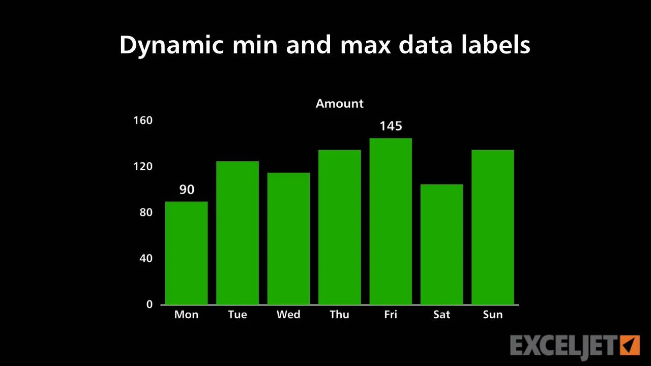
Dynamic min and max data labels
Using Conditional Formatting to Identify Date-Based Patterns in Excel In the New Formatting Rule box, select "Use a formula to determine which cells to format" as the rule type. Choose "Use a formula to determine which cells to format" to set custom date-based formatting. Enter the formula for the dates you want to highlight in the following format: "=TODAY ()-A1>X" where A1 is the cell number of the first cell ...

Solved: Bar Chart Data Labels - Conditional Formatting - W ...
How To Use Conditional Formatting in Excel in 5 Steps 4. Select an option from the drop-down menu. Once you select the "Conditional Formatting" button, Excel displays several options, starting with "Highlight Cells Rules" and ending with "Manage Rules." Selecting one option from the first five allows you to develop rules based on the option you choose.

Change color of data label placed, using the 'best fit ...
Conditional formatting for Data Labels in Power BI Where you can find the conditional formatting options? Select the visual > Go to the formatting pane> under Data labels > Values > Color Data Labels Let's Get Started- Add one line chart visual into page and create two measure for Profit & Sales. Note: If you don't want to create measure then you can directly use Sales and Profit fields.
Simple Conditional Formatting in Tableau - TAR Solutions
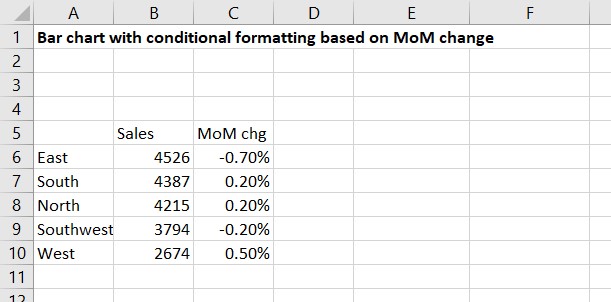
Excel bar chart with conditional formatting based on MoM ...

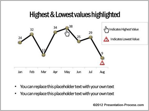
Highlight Max & Min Values in an Excel Line Chart - Xelplus ...
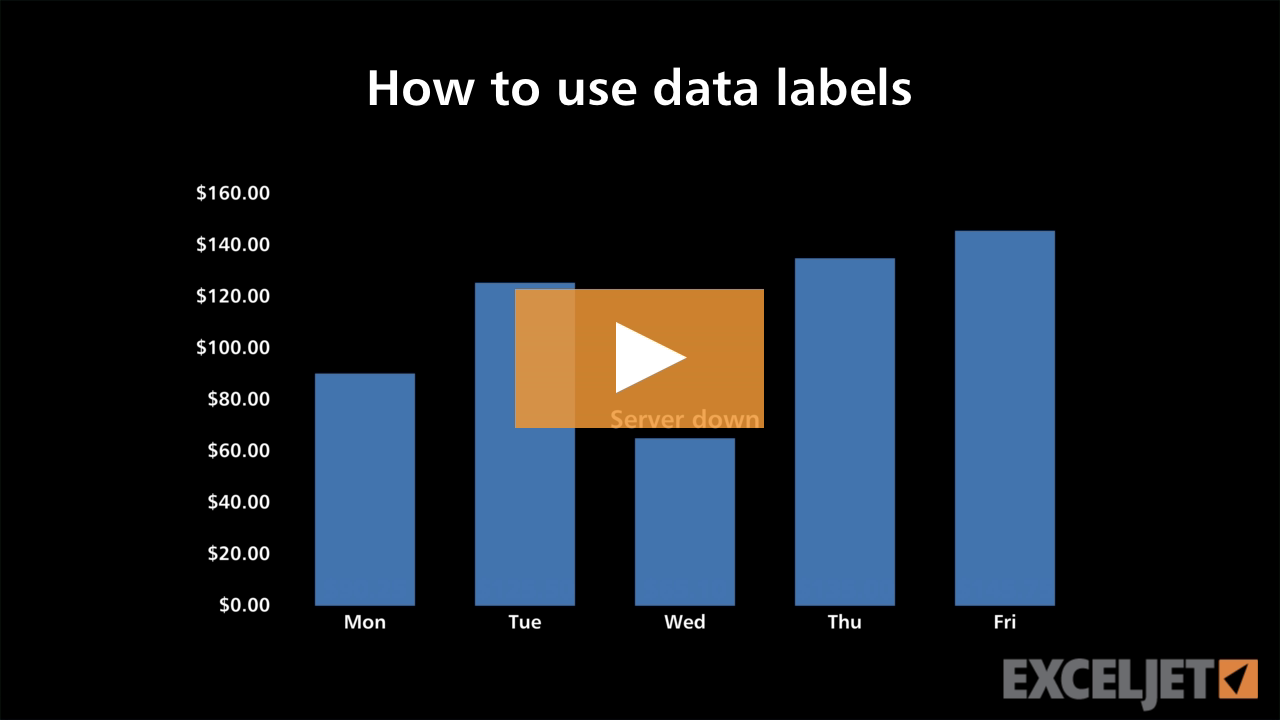
Excel tutorial: How to use data labels
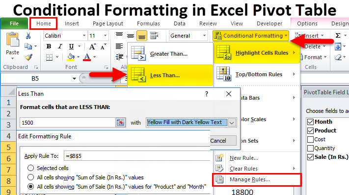
Conditional Formatting in Pivot Table (Example) | How To Apply?

Color Negative Chart Data Labels in Red with downward arrow

How to make a pie chart in Excel

Apply Custom Data Labels to Charted Points - Peltier Tech
Excel Bar Graph Color with Conditional Formatting (3 Suitable ...
Excel bar chart with conditional formatting based on MoM ...
Magical Conditional Formatting of Charts in PowerPoint

Power BI Conditional Formatting For Bar Chart Visuals ...

Dynamic Number Format for Millions and Thousands - PK: An ...
Conditional Formatting of Excel Charts - Peltier Tech

Highlight Max & Min Values in an Excel Line Chart - Xelplus ...
How to Use Conditional Formatting in Excel Online
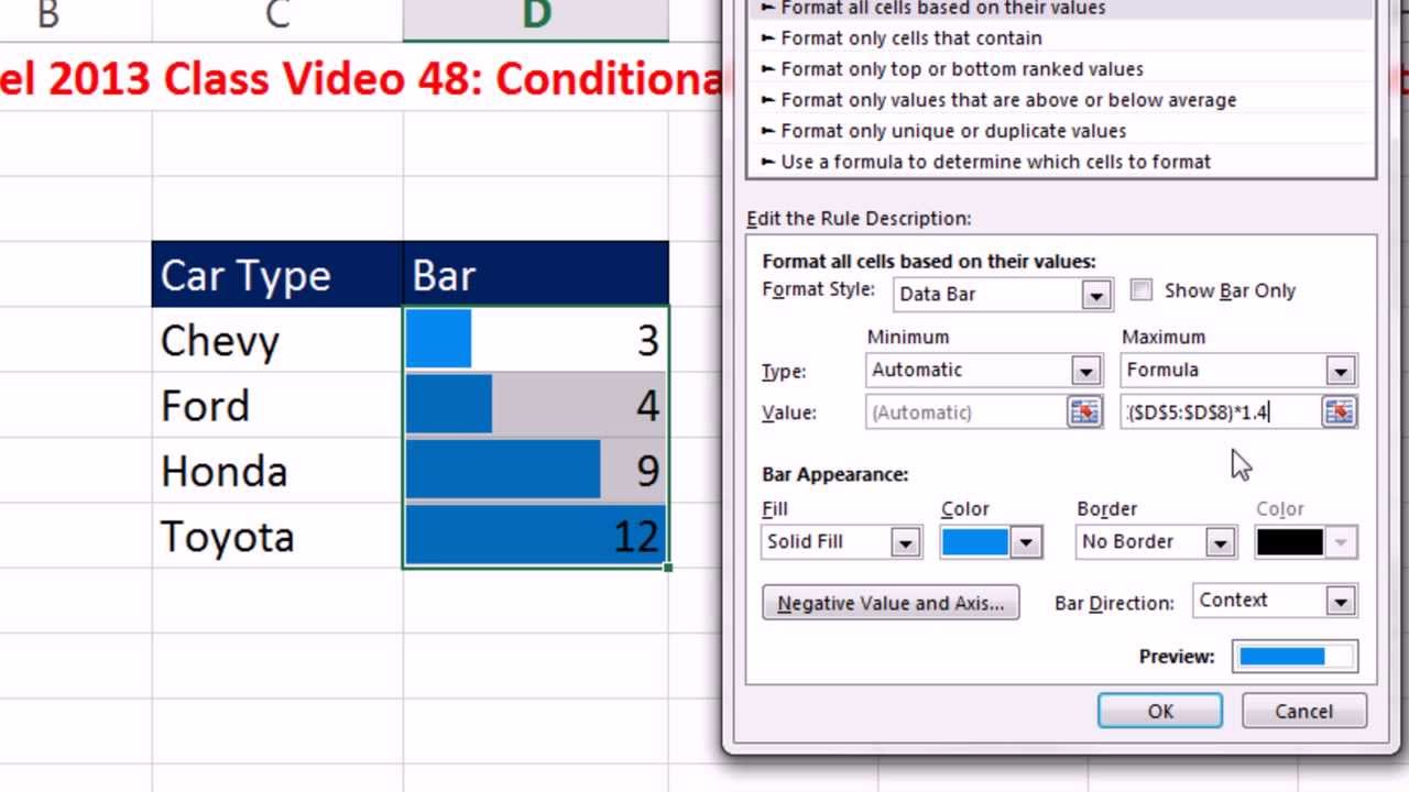
Highline Excel 2013 Class Video 48: Conditional Formatting: Bar Chart with Data Labels
Power BI Dynamic Conditional Formatting

Custom data labels in a chart
How to Create Excel Charts (Column or Bar) with Conditional ...
How to add a text label in the chart of MS Excel - Quora
Example: Charts with Data Labels — XlsxWriter Documentation

Conditional formatting for Data label colors at li ...
Power BI: Conditional formatting and data colors in action

Apply Custom Conditional Formatting to Clustered Column Chart ...
Excel bar chart with conditional formatting based on MoM ...
How to change chart axis labels' font color and size in Excel?

Formatting Charts in Excel - GeeksforGeeks
Post a Comment for "42 conditional formatting data labels excel"